In this article, we will demonstrate the use of color schemes in tidyplots. We will explore the default color schemes that come with tidyplots and are ready to use for plotting. These include schemes for discrete, continuous and diverging variables. To conclude, we will discuss the creation of custom color schemes from hex values.
Default color schemes
tidyplots comes with a number of default color schemes. Many of them
are adapted from the viridisLite and
RColorBrewer packages. You access them by loading the the
tidyplots library and start typing colors_. The
auto-completion will guide you through a selection of
discrete, continuous and
diverging schemes.
Let’s have a look at the signature scheme of tidyplots
colors_discrete_friendly, which was designed to work well
for people with color vision deficiency. When running the line
colors_discrete_friendly in the console or within a script,
a preview of the scheme will be rendered to the Viewer pane in the lower
right of the RStudio Desktop interface.
In essence, tidyplots color schemes are just a character vector of hex colors with a special print method that sends a preview to the RStudio viewer pane.
colors_discrete_friendly
A tidyplots color scheme with 6 colors.c(
"#0072B2","#56B4E9","#009E73","#F5C710","#E69F00","#D55E00")
Tip: You can copy individual hex colors directly from the preview to use them in your script.
Discrete
Discrete color schemes are meant for categorical variables. The default schemes in tidyplots consist of 5–7 colors. However, if more categories are present in the plot, tidyplots will automatically fill up the gaps between colors to deliver exactly the number that is required for the plot.
Similarly, when more colors are provided than needed, tidyplots will select the required number of colors by attempting to evenly sample from the supplied color vector.
energy |>
  tidyplot(year, energy, color = energy_source) |>
  add_barstack_absolute()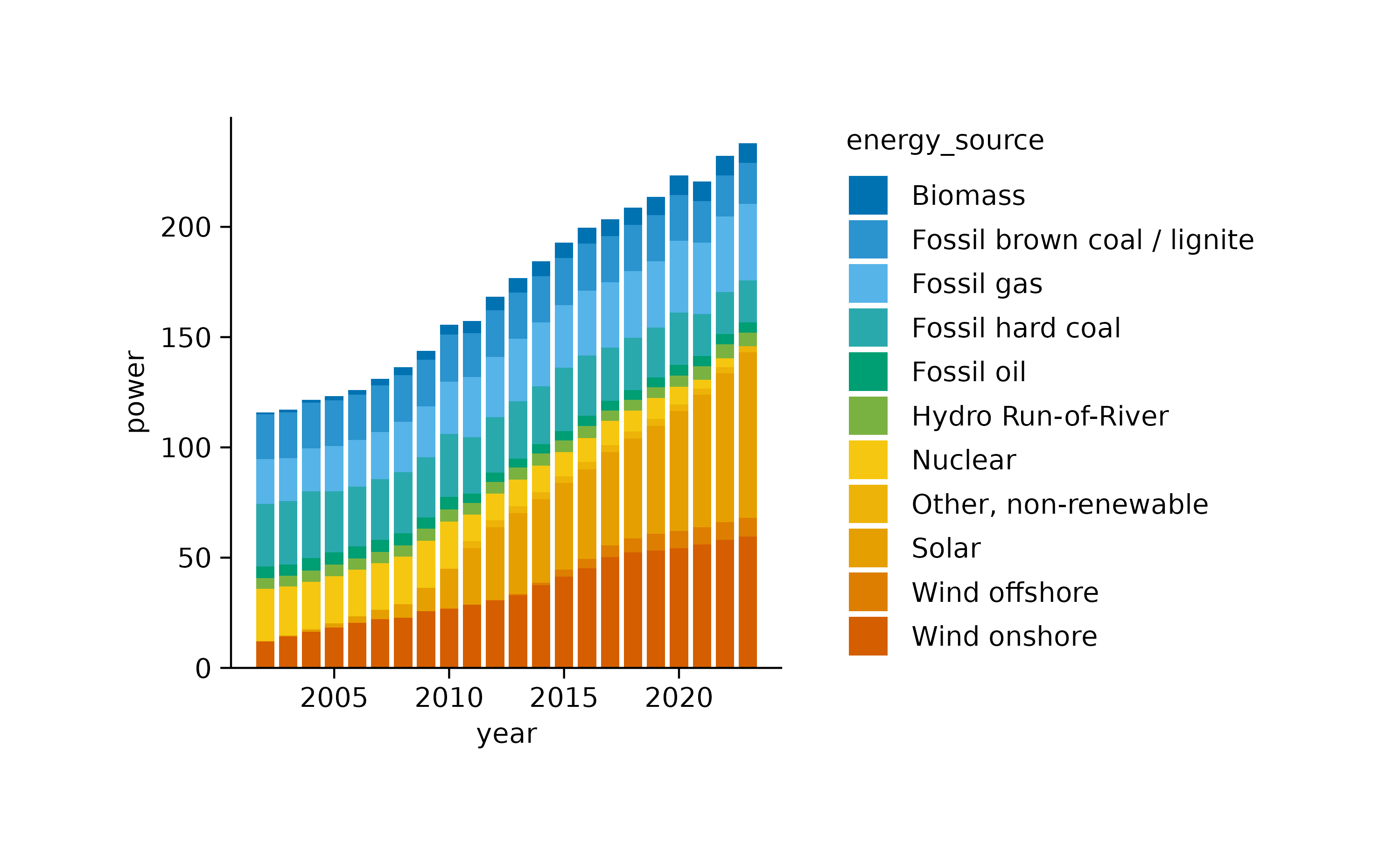
And here are some alternative color schemes.
energy |>
  tidyplot(year, energy, color = energy_source) |>
  add_barstack_absolute() |>
  adjust_colors(colors_discrete_seaside)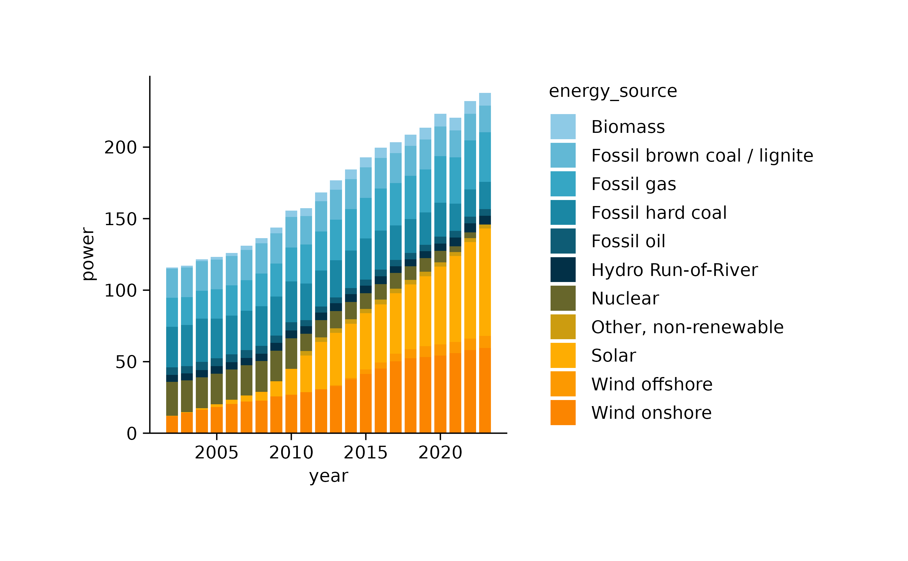
energy |>
  tidyplot(year, energy, color = energy_source) |>
  add_barstack_absolute() |>
  adjust_colors(colors_discrete_friendly_long)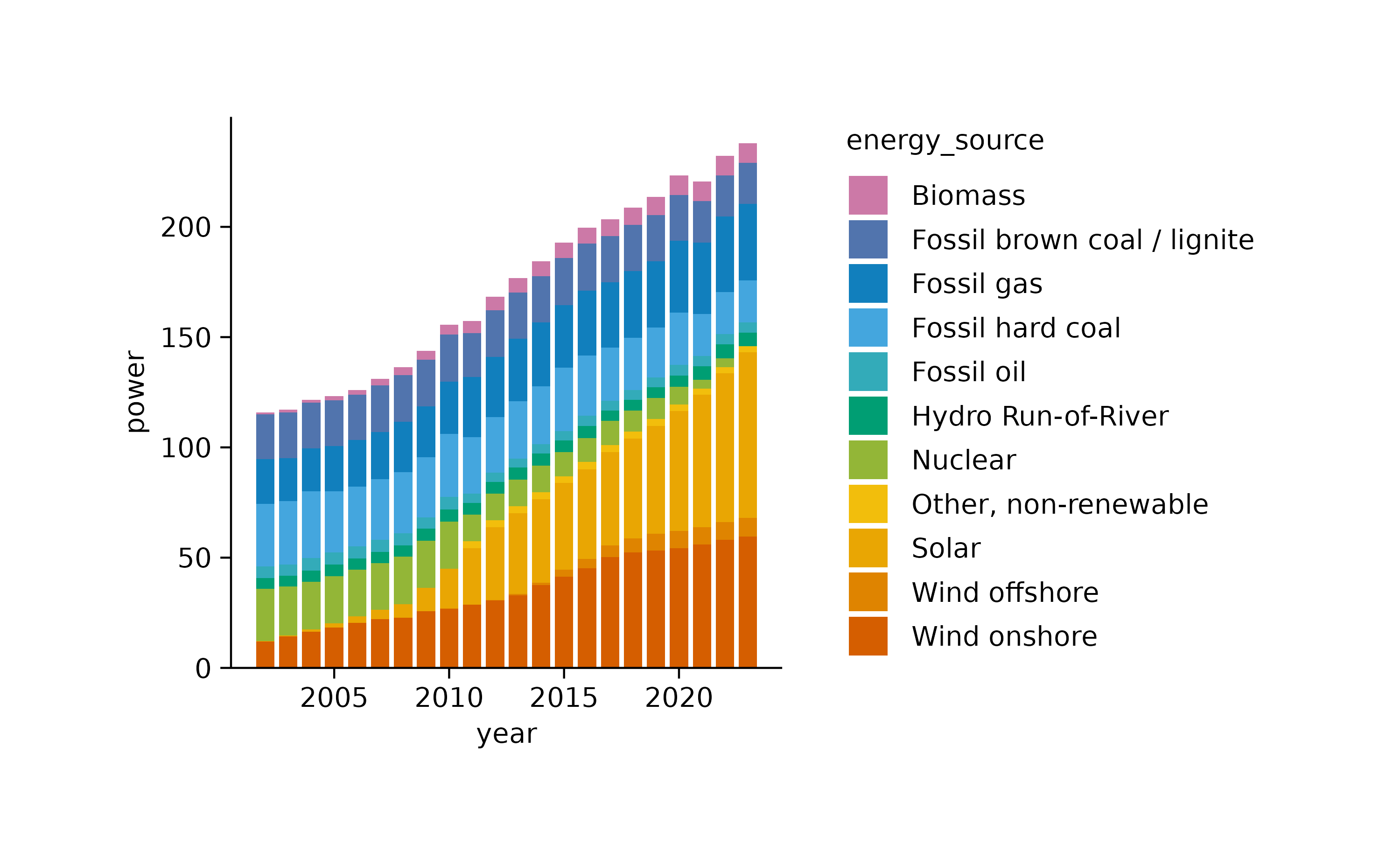
energy |>
  tidyplot(year, energy, color = energy_source) |>
  add_barstack_absolute() |>
  adjust_colors(colors_discrete_apple)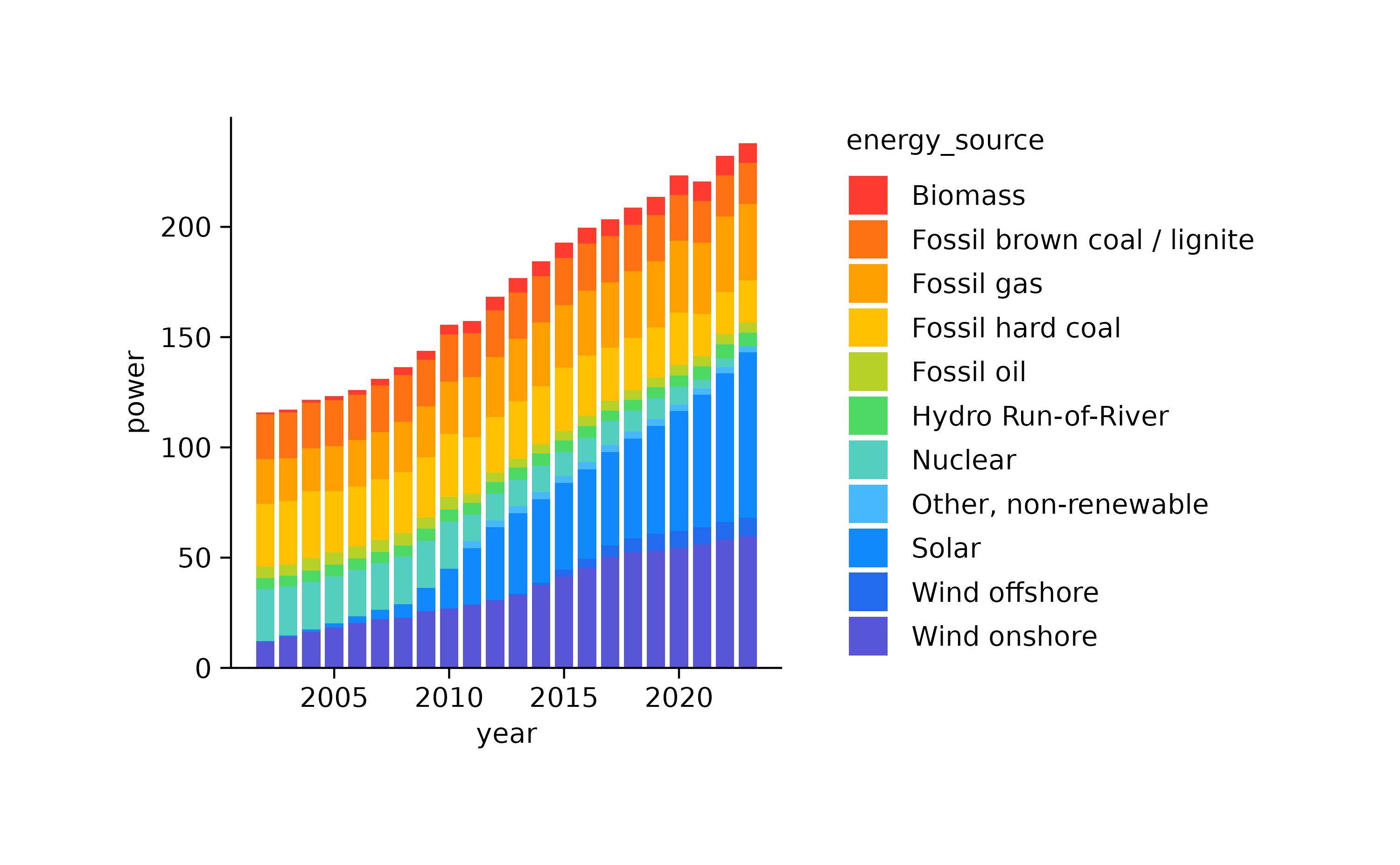
energy |>
  tidyplot(year, energy, color = energy_source) |>
  add_barstack_absolute() |>
  adjust_colors(colors_discrete_ibm)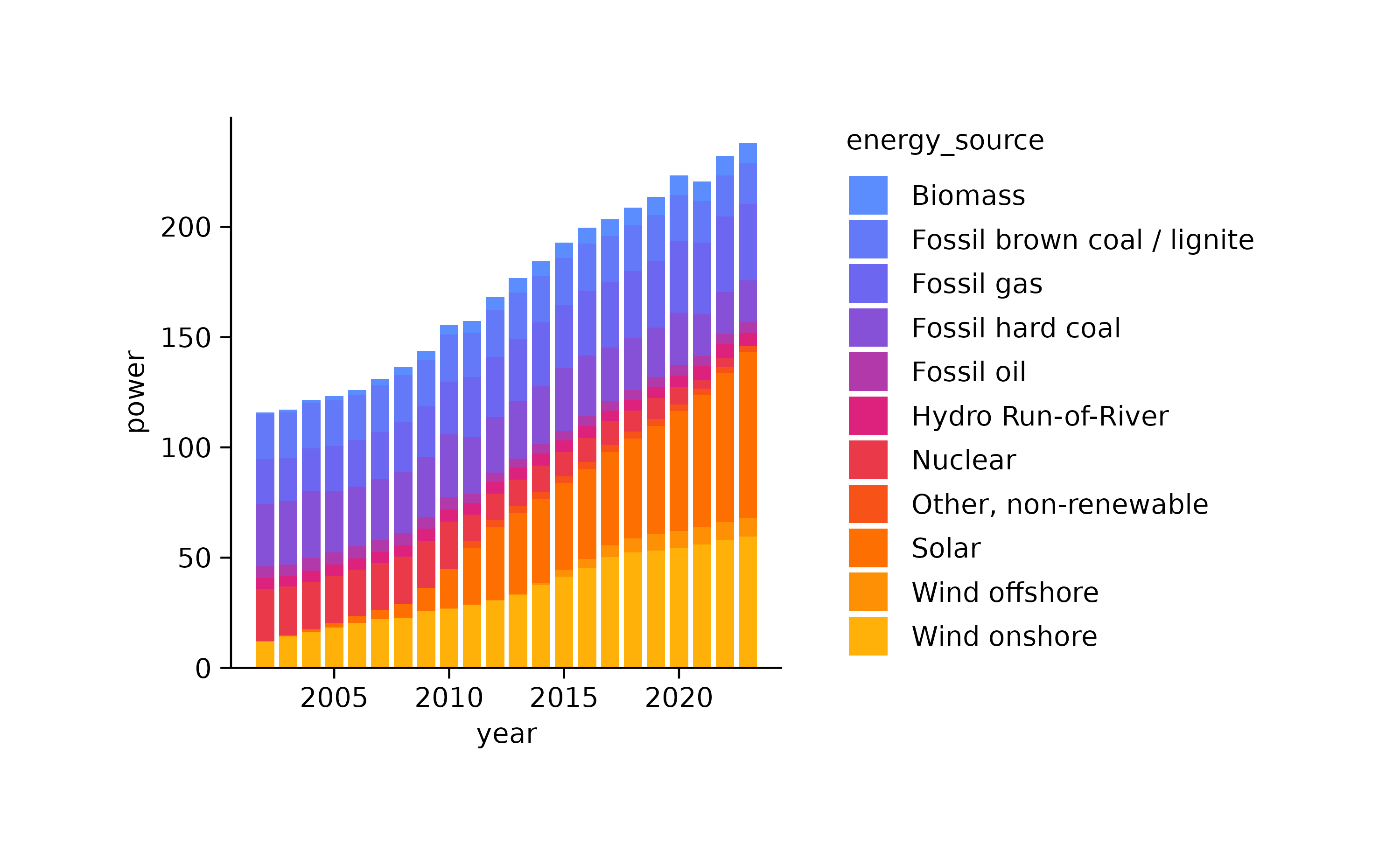
energy |>
  tidyplot(year, energy, color = energy_source) |>
  add_barstack_absolute() |>
  adjust_colors(colors_discrete_candy)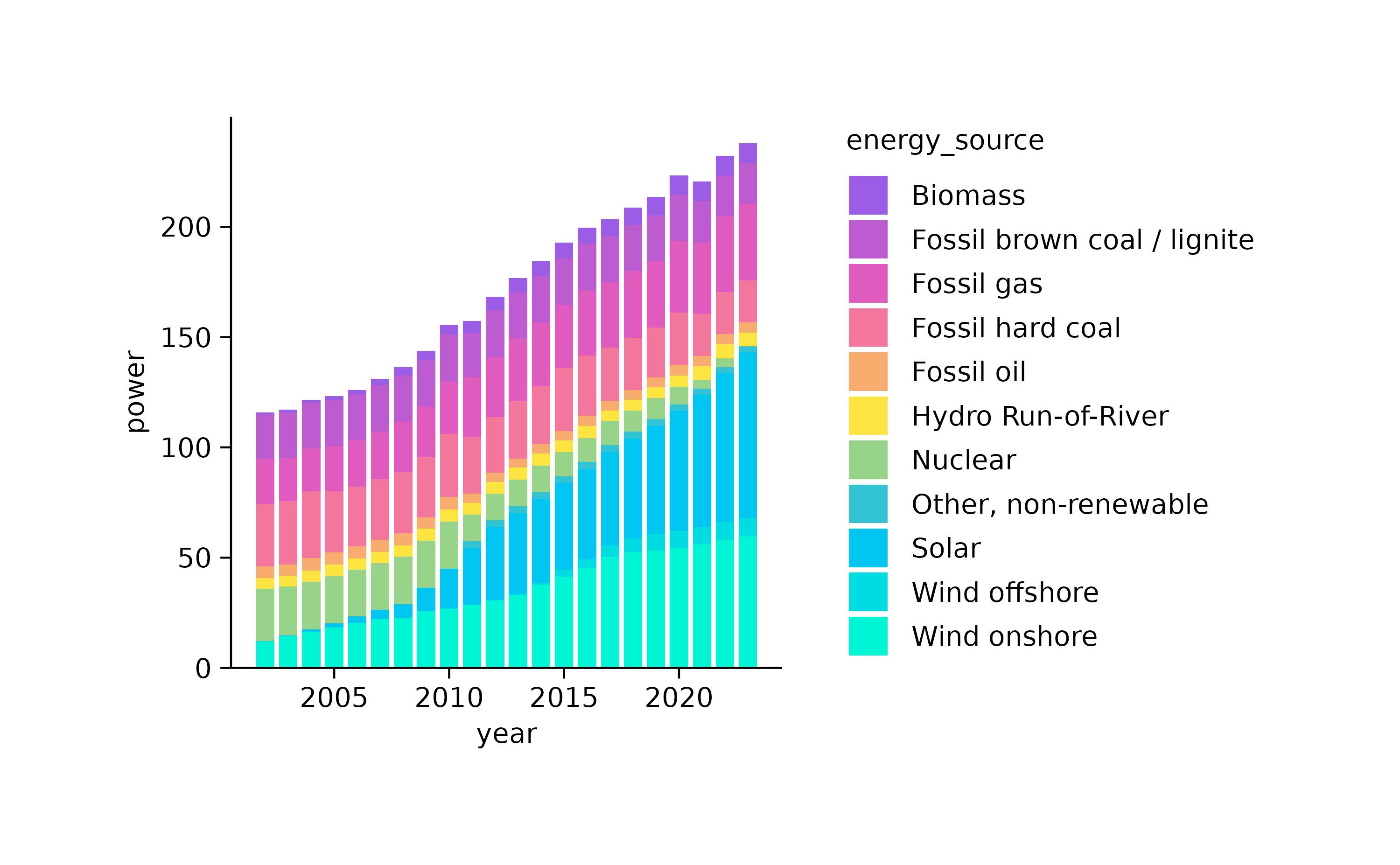
energy |>
  tidyplot(year, energy, color = energy_source) |>
  add_barstack_absolute() |>
  adjust_colors(colors_discrete_alger)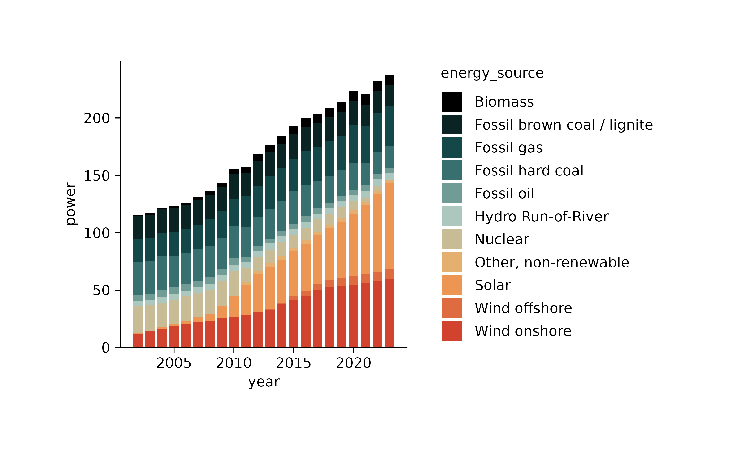
energy |>
  tidyplot(year, energy, color = energy_source) |>
  add_barstack_absolute() |>
  adjust_colors(colors_discrete_rainbow)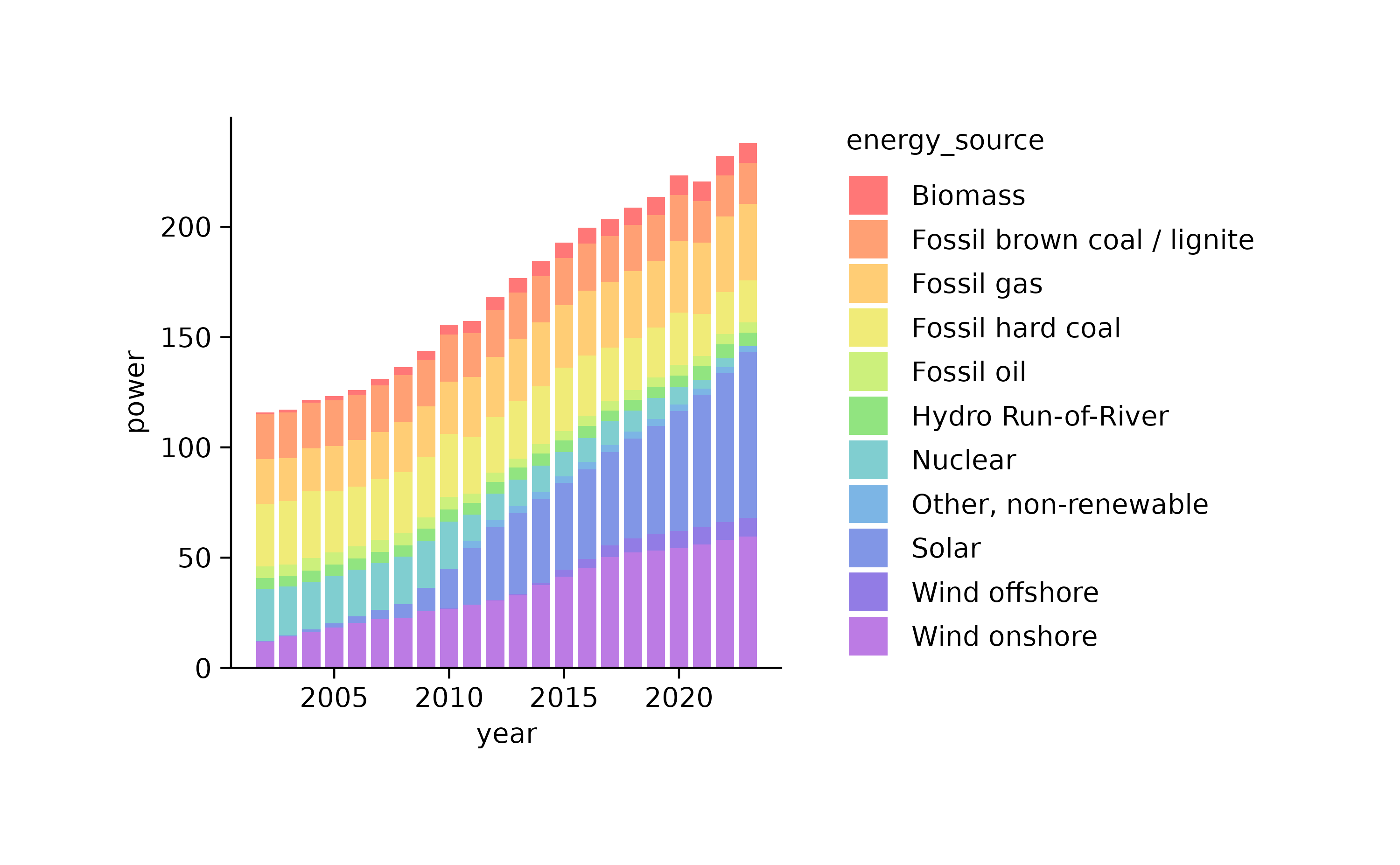
Continuous
Continuous color schemes are meant for continuous variables. The default schemes in tidyplots usually consist of 265 colors.
colors_continuous_viridiscolors_continuous_viridis
A tidyplots color scheme with 265 colors, downsampled to 42 colors.c(
"#440154FF","#460A5DFF","#471264FF","#481B6DFF","#482374FF","#472C7AFF","#46337FFF","#443A83FF","#424186FF","#3F4889FF","#3C508BFF","#39568CFF","#365D8DFF","#33638DFF","#306A8EFF","#2D708EFF","#2B758EFF","#297B8EFF","#26818EFF","#24878EFF","#228D8DFF","#20928CFF","#1F988BFF","#1F9F88FF","#20A486FF","#24AA83FF","#29AF7FFF","#31B57BFF","#3BBB75FF","#45C06FFF","#53C569FF","#5EC962FF","#6ECE58FF","#7BD250FF","#8AD647FF","#9CD93CFF","#AADC32FF","#BDDF26FF","#CCE11EFF","#DEE318FF","#EDE51BFF","#FDE725FF")
Here is a use case for a continuous color scheme.
climate |>
  tidyplot(x = month, y = year, color = max_temperature) |>
  add_heatmap()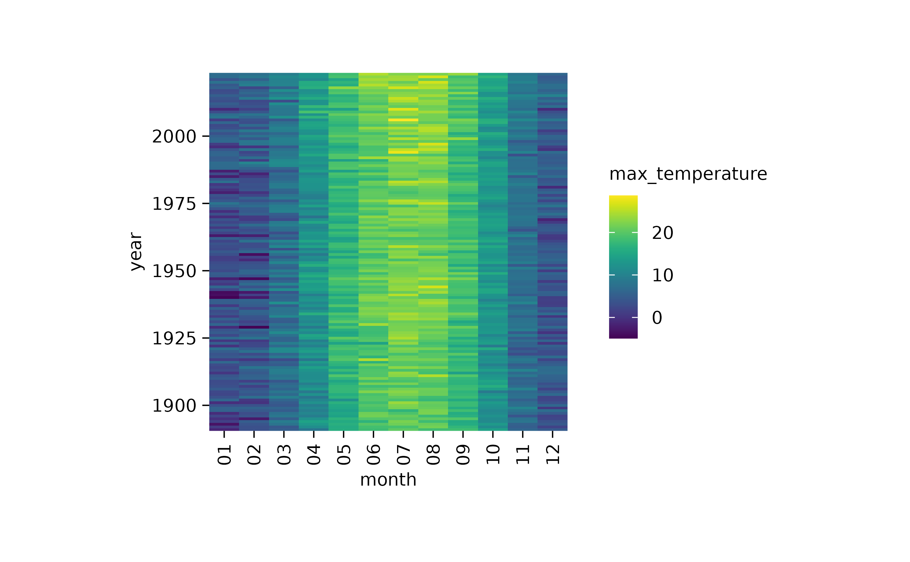
And here are some alternative color schemes.
climate |>
  tidyplot(x = month, y = year, color = max_temperature) |>
  add_heatmap() |>
  adjust_colors(new_colors = colors_continuous_inferno)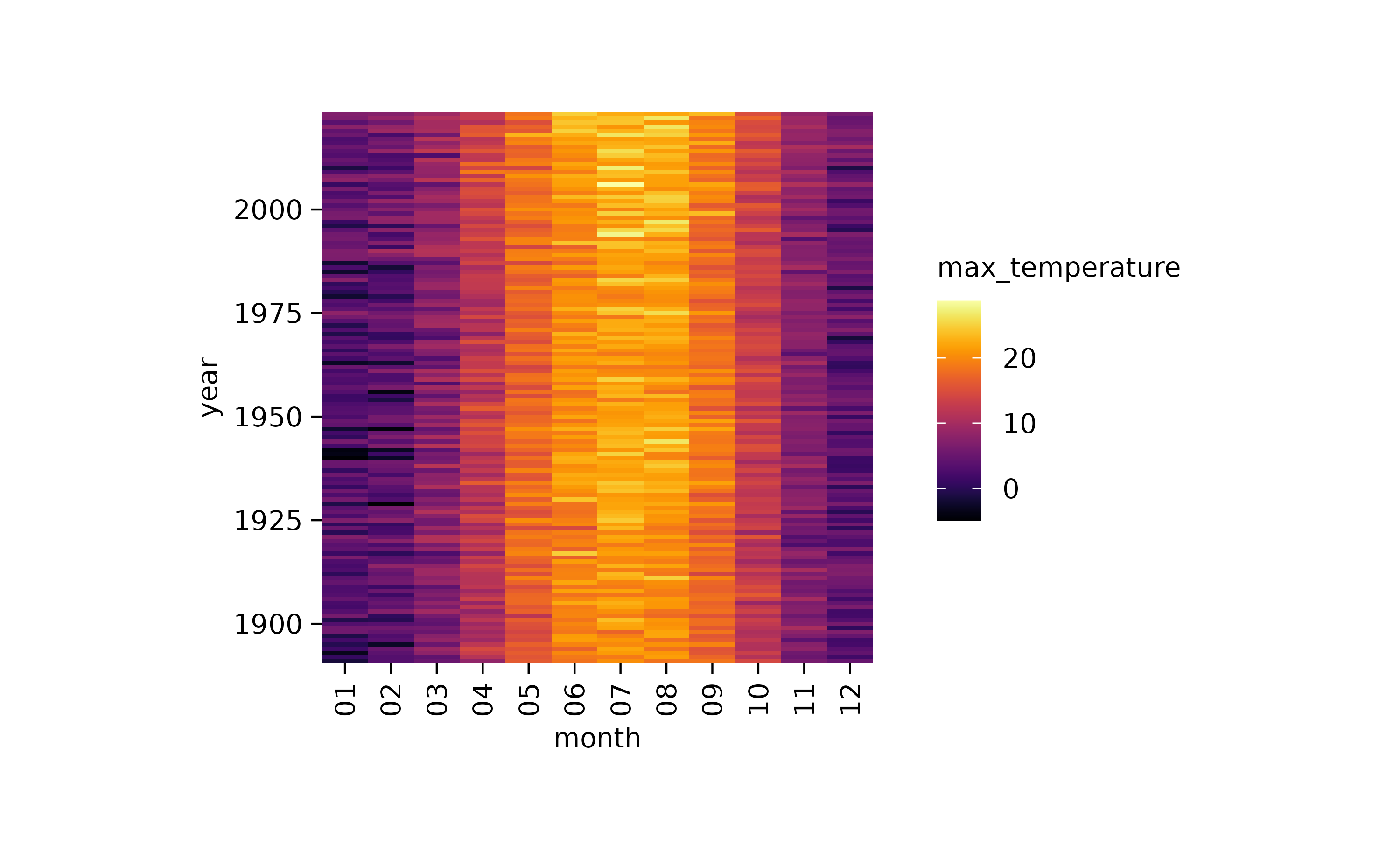
climate |>
  tidyplot(x = month, y = year, color = max_temperature) |>
  add_heatmap() |>
  adjust_colors(new_colors = colors_continuous_mako)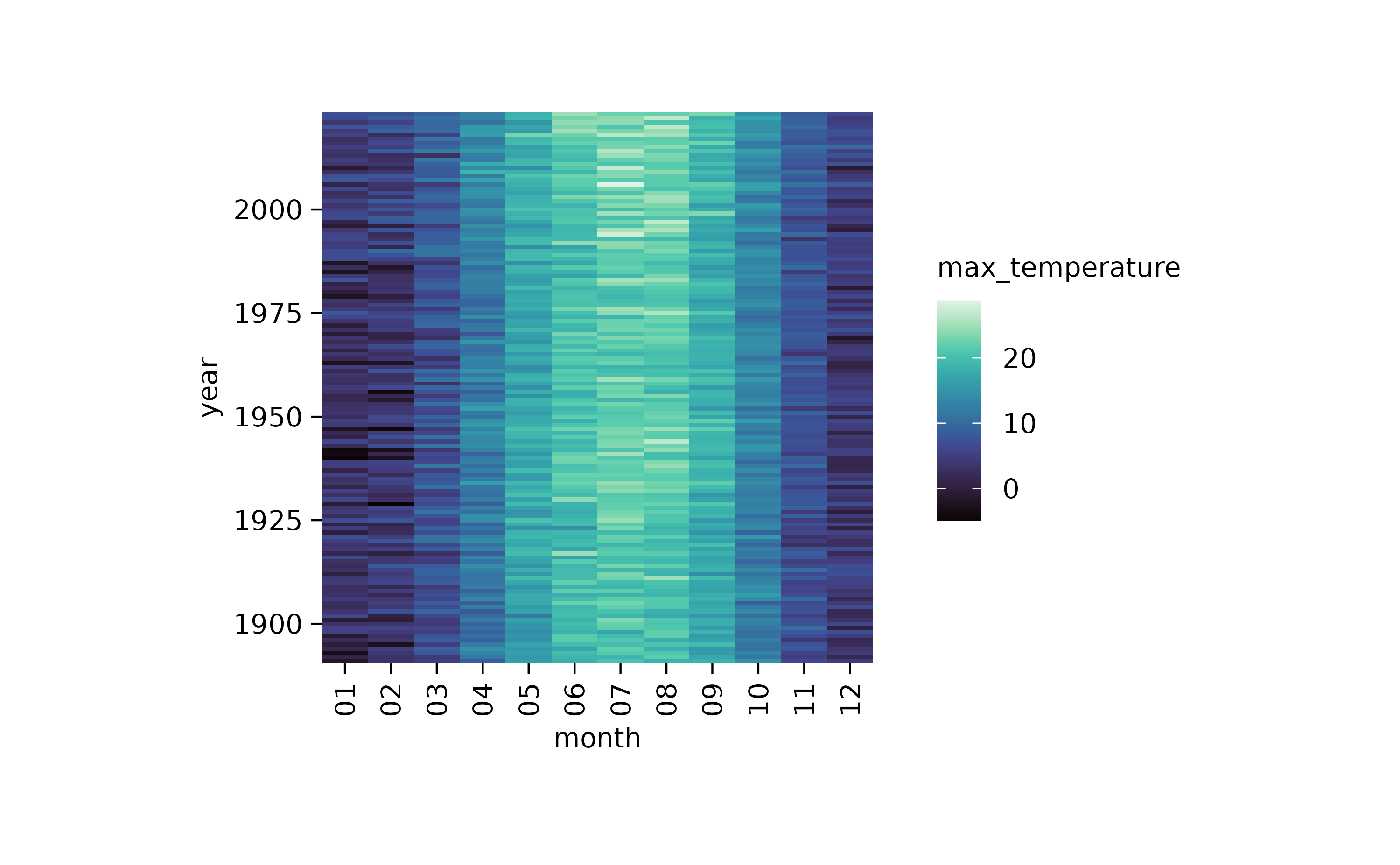
climate |>
  tidyplot(x = month, y = year, color = max_temperature) |>
  add_heatmap() |>
  adjust_colors(new_colors = colors_continuous_turbo)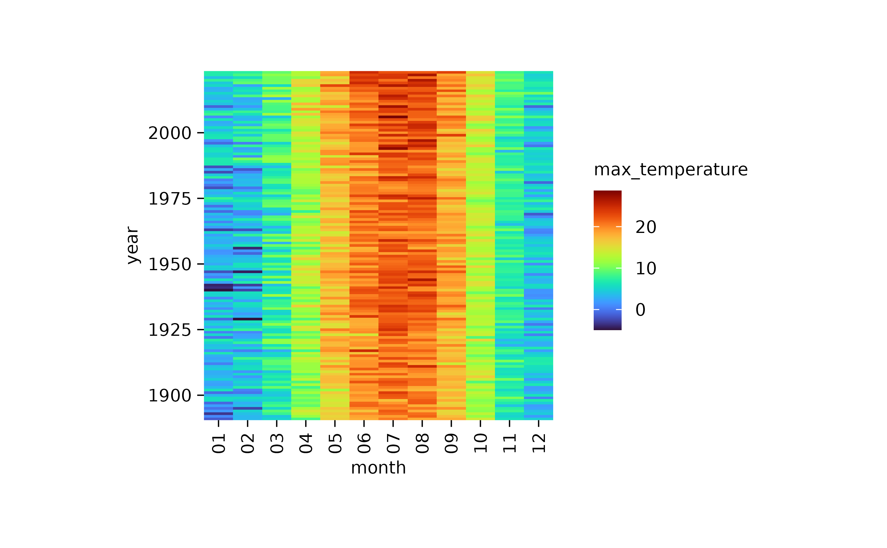
climate |>
  tidyplot(x = month, y = year, color = max_temperature) |>
  add_heatmap() |>
  adjust_colors(new_colors = colors_continuous_rocket)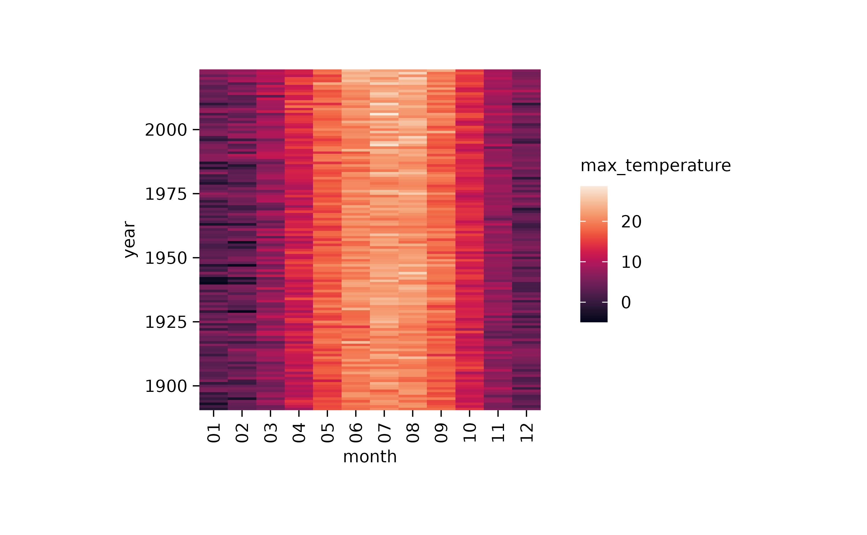
Diverging
Diverging color schemes are meant for continuous variables that have a central point in the middle. A classical example is the blue–white–red gradient used for gene expression heatmaps.
colors_diverging_blue2redcolors_diverging_blue2red
A tidyplots color scheme with 17 colors.c(
"#0000FF","#1F1FFF","#3F3FFF","#5F5FFF","#7F7FFF","#9F9FFF","#BFBFFF","#DFDFFF","#FFFFFF","#FFDFDF","#FFBFBF","#FF9F9F","#FF7F7F","#FF5F5F","#FF3F3F","#FF1F1F","#FF0000")
Here is a use case for a diverging color scheme.
gene_expression |>
  tidyplot(x = sample, y = external_gene_name, color = expression) |>
  add_heatmap(scale = "row") |>
  sort_y_axis_labels(direction) |>
  adjust_size(height = 100)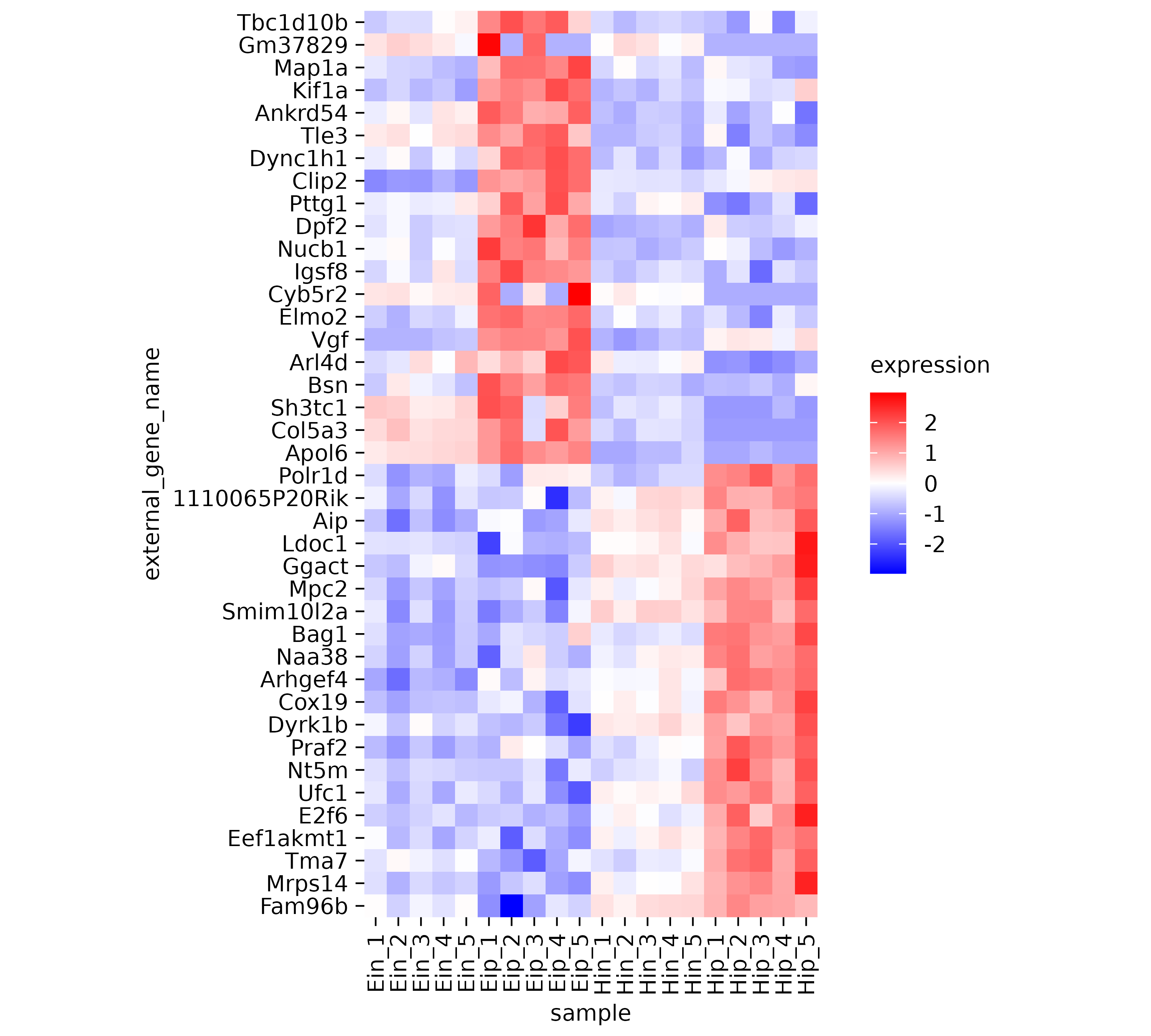
And here are some alternative color schemes.
gene_expression |>
  tidyplot(x = sample, y = external_gene_name, color = expression) |>
  add_heatmap(scale = "row") |>
  sort_y_axis_labels(direction) |>
  adjust_size(height = 100) |>
  adjust_colors(new_colors = colors_diverging_blue2brown)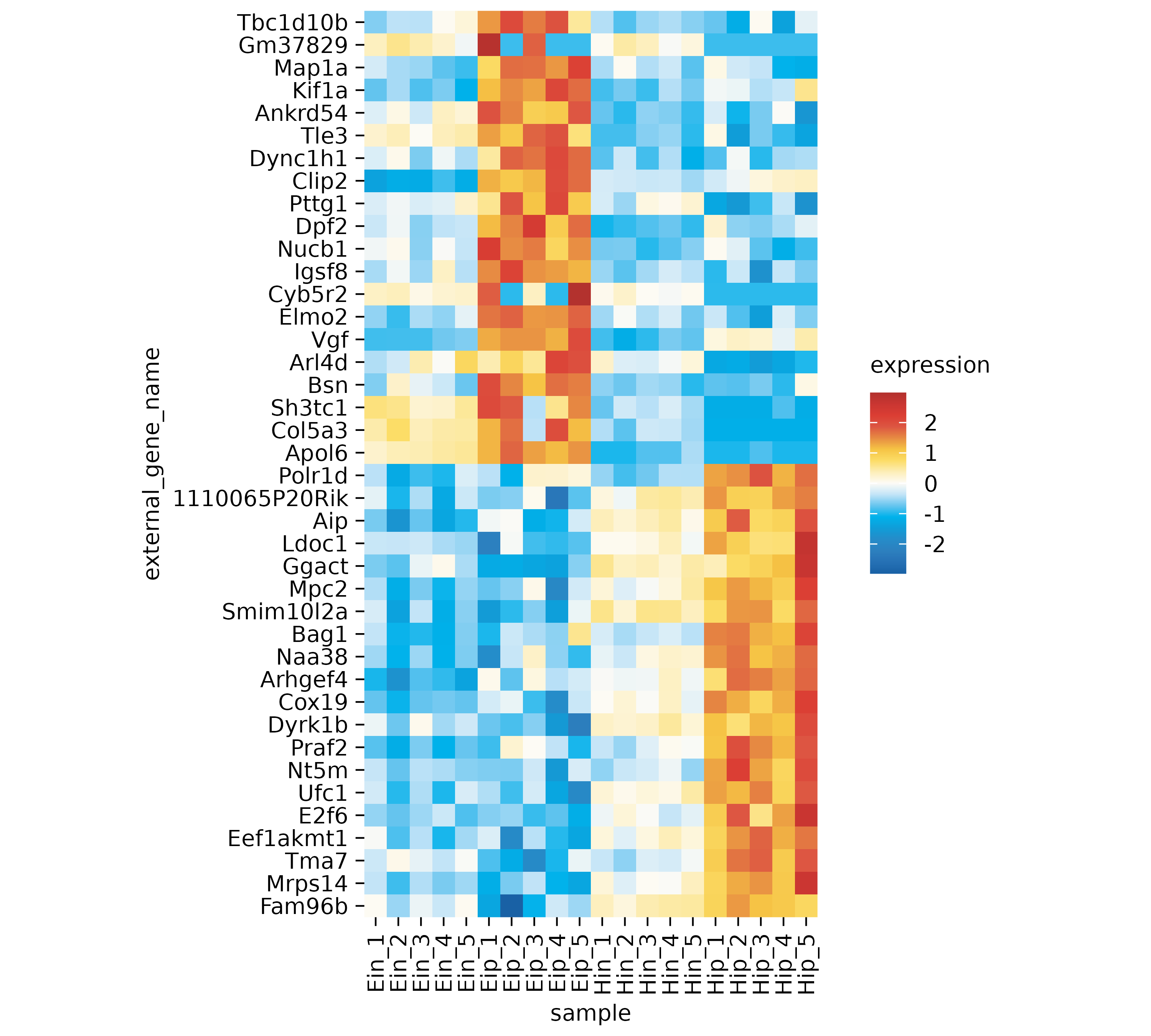
gene_expression |>
  tidyplot(x = sample, y = external_gene_name, color = expression) |>
  add_heatmap(scale = "row") |>
  sort_y_axis_labels(direction) |>
  adjust_size(height = 100) |>
  adjust_colors(new_colors = colors_diverging_spectral)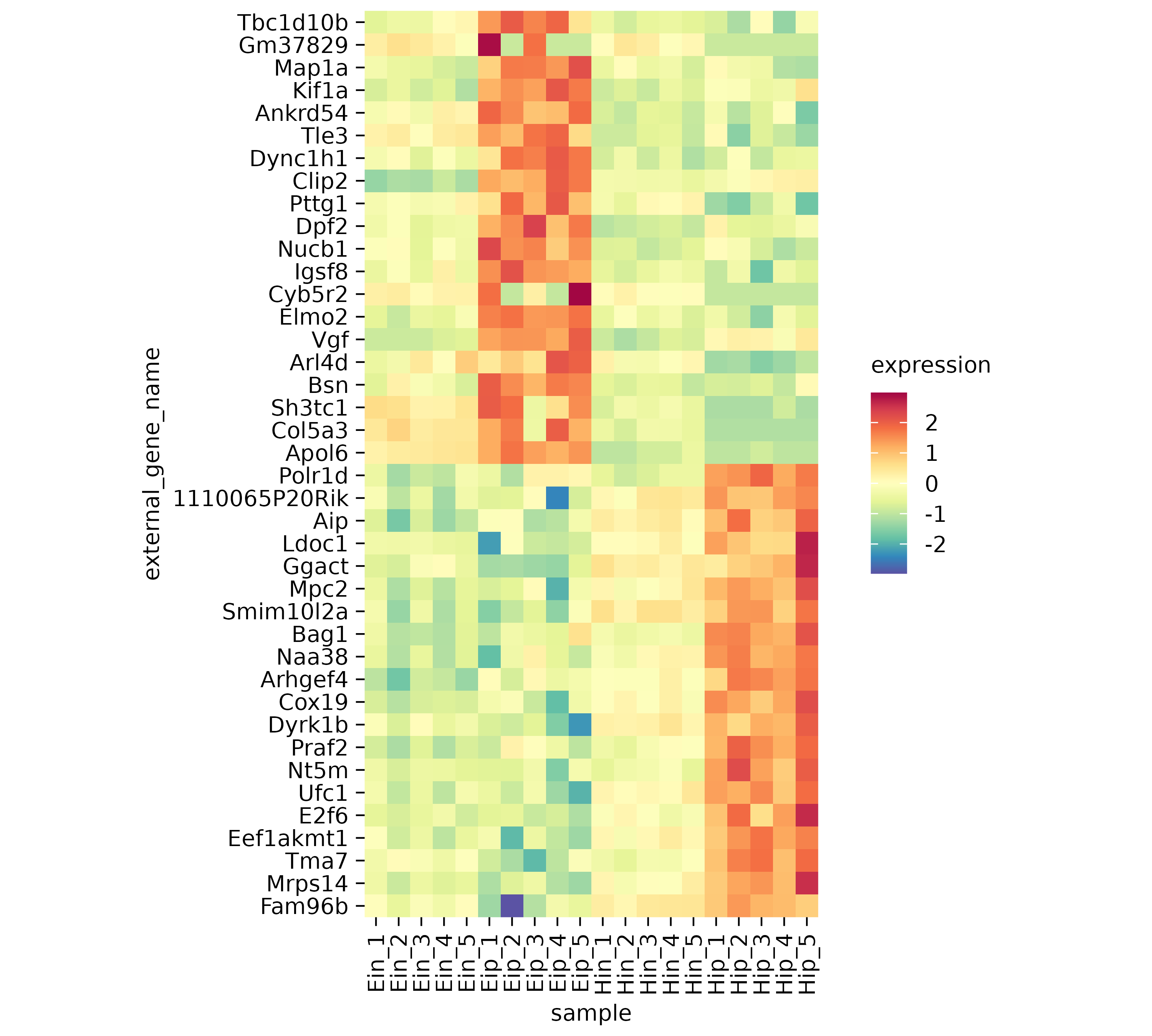
gene_expression |>
  tidyplot(x = sample, y = external_gene_name, color = expression) |>
  add_heatmap(scale = "row") |>
  sort_y_axis_labels(direction) |>
  adjust_size(height = 100) |>
  adjust_colors(new_colors = colors_diverging_icefire)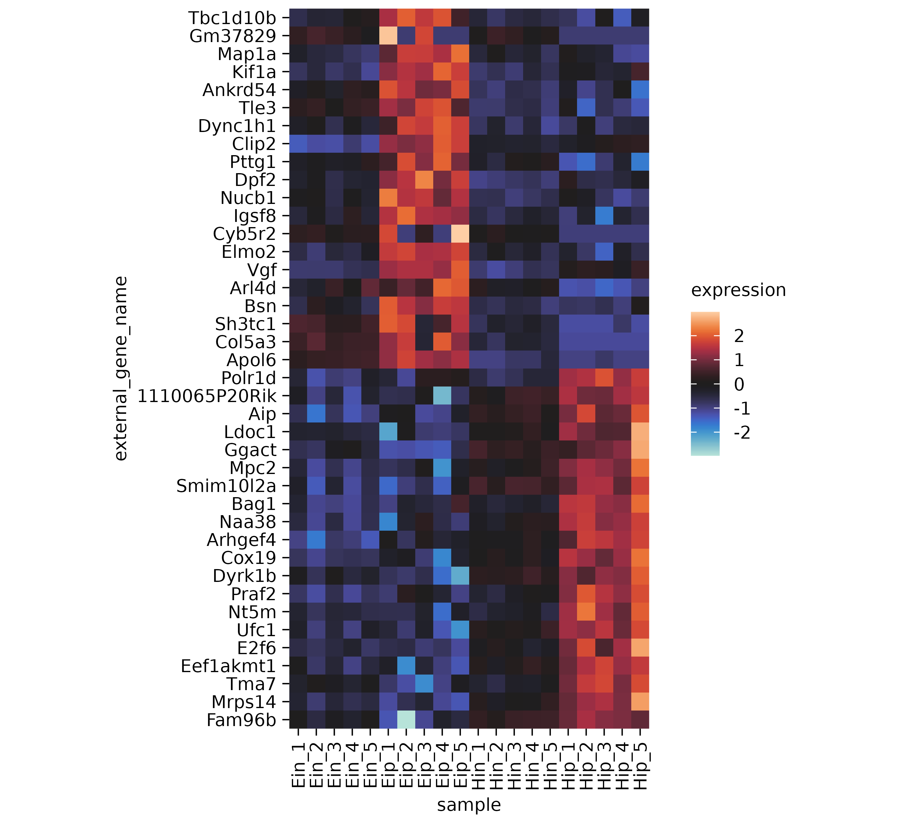
Custom color schemes
Of course you can also construct custom color schemes using the
new_color_scheme() function.
my_colors <-
  new_color_scheme(c("#ECA669","#E06681","#8087E2","#E2D269"),
                   name = "my_custom_color_scheme")
my_colors
my_custom_color_scheme
A tidyplots color scheme with 4 colors.c(
"#ECA669","#E06681","#8087E2","#E2D269")
Than you can use your scheme as input to the
adjust_colors() function.
energy |>
  tidyplot(year, energy, color = energy_source) |>
  add_barstack_absolute() |>
  adjust_colors(new_colors = my_colors)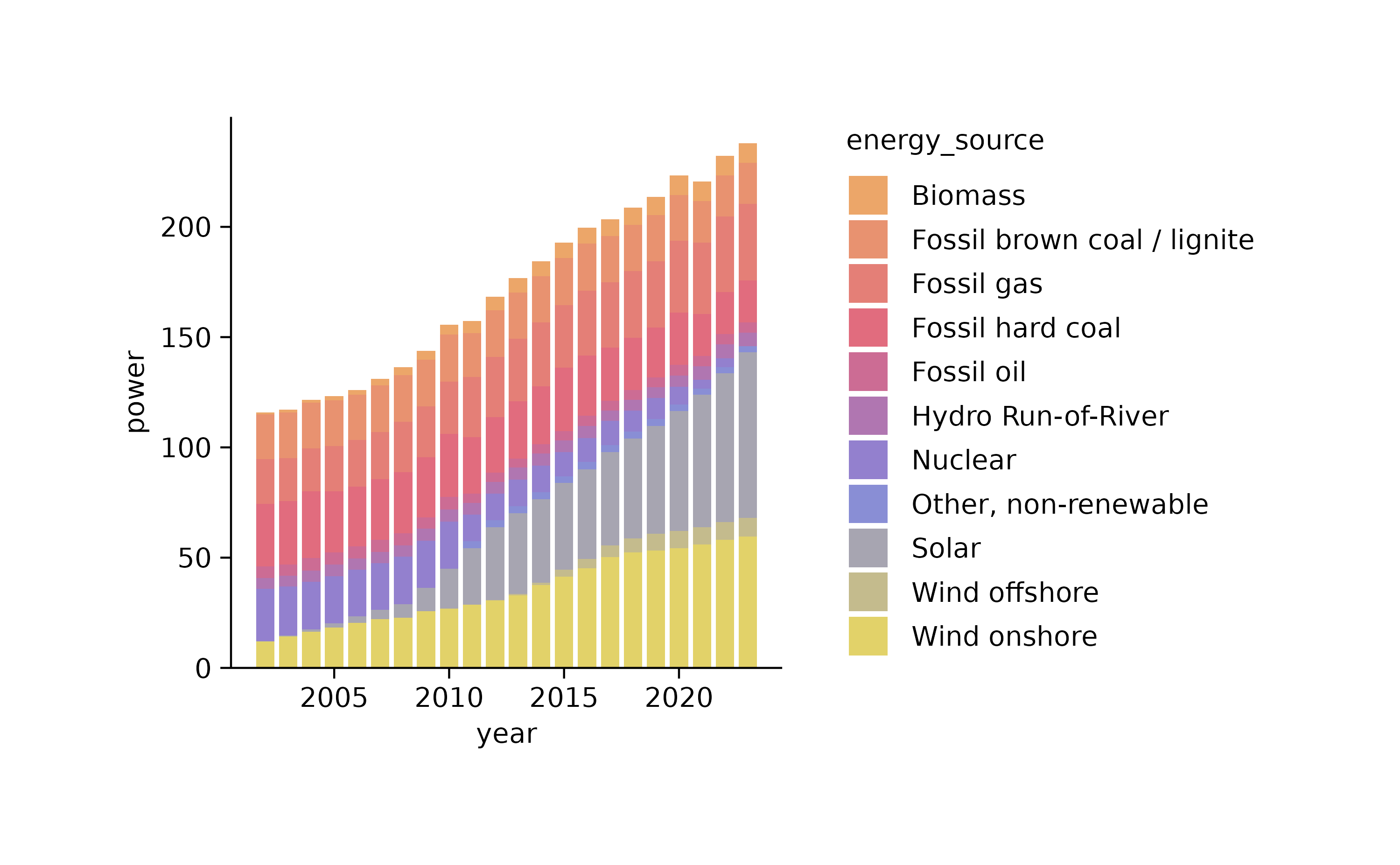
Besides creating new schemes, you can also subset and concatenate existing schemes in the exact same way you would do with a regular character string.
colors_discrete_metro[2]Untitled color scheme
A tidyplots color scheme with 1 colors.c(
"#4FAE62")
colors_discrete_metro[2:4]Untitled color scheme
A tidyplots color scheme with 3 colors.c(
"#4FAE62","#F6C54D","#E37D46")
c(colors_discrete_metro, colors_discrete_seaside)Untitled color scheme
A tidyplots color scheme with 10 colors.c(
"#4DACD6","#4FAE62","#F6C54D","#E37D46","#C02D45","#8ecae6","#219ebc","#023047","#ffb703","#fb8500")
What’s more?
To dive deeper into code-based plotting, here a couple of resources.
tidyplots documentation
Package index
Overview of all tidyplots functionsGet started
Getting started guideVisualizing data
Article with examples for common data visualizationsAdvanced plotting
Article about advanced plotting techniques and workflowsColor schemes
Article about the use of color schemes
Other resources
Hands-On Programming with R
Free online book by Garrett GrolemundR for Data Science
Free online book by Hadley WickhamFundamentals of Data Visualization
Free online book by Claus O. Wilke