The goal of bro_plot_heatmap() is to provide a tidyverse-style interface to the powerful heatmap package pheatmap by @raivokolde. Although heatmaps can be generated via ggplot2::geom_tile(), it is hard to reach the versatility and beauty of a genuine heatmap function like pheatmap::pheatmap().
Data requirements
bro_plot_heatmap() requires tidy data in long format, see tidyverse.
As an example we will use the gene expression data set bro_data_exprs. In the tidyverse lingo the columns of a data frame are called variables. One of these variables named expression contains the numeric values to be color-coded in the heatmap. Furthermore we will use the variables sample for heatmap columns and external_gene_name for heatmap rows.
bro_data_exprs
#> # A tibble: 800 x 12
#>    ensembl_gene_id    external_gene_na… Eip_vs_Hip.padj direction is_immune_gene
#>    <chr>              <chr>                       <dbl> <chr>     <chr>
#>  1 ENSMUSG00000033576 Apol6                    3.79e-28 up        no
#>  2 ENSMUSG00000033576 Apol6                    3.79e-28 up        no
#>  3 ENSMUSG00000033576 Apol6                    3.79e-28 up        no
#>  4 ENSMUSG00000033576 Apol6                    3.79e-28 up        no
#>  5 ENSMUSG00000033576 Apol6                    3.79e-28 up        no
#>  6 ENSMUSG00000033576 Apol6                    3.79e-28 up        no
#>  7 ENSMUSG00000033576 Apol6                    3.79e-28 up        no
#>  8 ENSMUSG00000033576 Apol6                    3.79e-28 up        no
#>  9 ENSMUSG00000033576 Apol6                    3.79e-28 up        no
#> 10 ENSMUSG00000033576 Apol6                    3.79e-28 up        no
#> # … with 790 more rows, and 7 more variables: count_type <chr>, group <chr>,
#> #   replicate <chr>, expression <dbl>, sample <chr>, sample_type <chr>,
#> #   condition <chr>

glimpse(bro_data_exprs)
#> Rows: 800
#> Columns: 12
#> $ ensembl_gene_id    <chr> "ENSMUSG00000033576", "ENSMUSG00000033576", "ENSMUS…
#> $ external_gene_name <chr> "Apol6", "Apol6", "Apol6", "Apol6", "Apol6", "Apol6…
#> $ Eip_vs_Hip.padj    <dbl> 3.793735e-28, 3.793735e-28, 3.793735e-28, 3.793735e…
#> $ direction          <chr> "up", "up", "up", "up", "up", "up", "up", "up", "up…
#> $ is_immune_gene     <chr> "no", "no", "no", "no", "no", "no", "no", "no", "no…
#> $ count_type         <chr> "vsd", "vsd", "vsd", "vsd", "vsd", "vsd", "vsd", "v…
#> $ group              <chr> "Hin", "Hin", "Hin", "Hin", "Hin", "Ein", "Ein", "E…
#> $ replicate          <chr> "1", "2", "3", "4", "5", "1", "2", "3", "4", "5", "…
#> $ expression         <dbl> 2.203755, 2.203755, 2.660558, 2.649534, 3.442740, 5…
#> $ sample             <chr> "Hin_1", "Hin_2", "Hin_3", "Hin_4", "Hin_5", "Ein_1…
#> $ sample_type        <chr> "input", "input", "input", "input", "input", "input…
#> $ condition          <chr> "healthy", "healthy", "healthy", "healthy", "health…
Basic usage
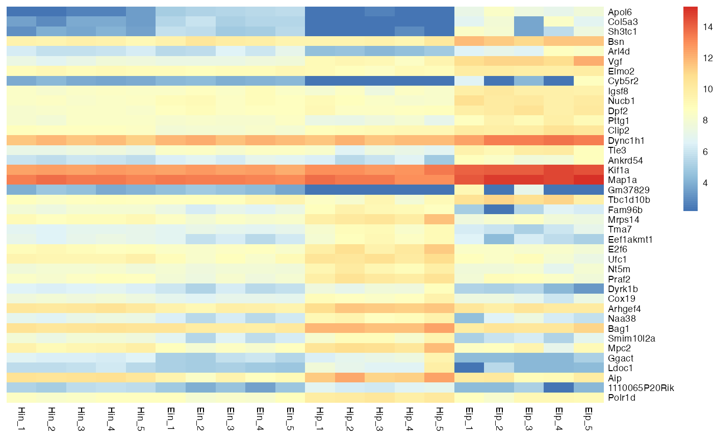
The basic layout of the heatmap relies on the parameters rows, columns and values. You can think of them like aesthetics in ggplot2::ggplot(), similar to something like aes(x = columns, y = rows, fill = values).
bro_plot_heatmap(bro_data_exprs,
                 rows = external_gene_name,
                 columns = sample,
                 values = expression
)
Features
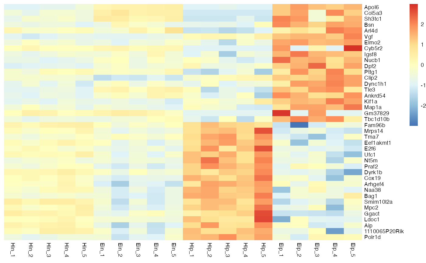
Data scaling
With the parameter scale you can activate data scaling for "row" or "column". By default data scaling is turned off scale = "none".
bro_plot_heatmap(bro_data_exprs,
                 rows = external_gene_name,
                 columns = sample,
                 values = expression,
                 scale = "row"
)
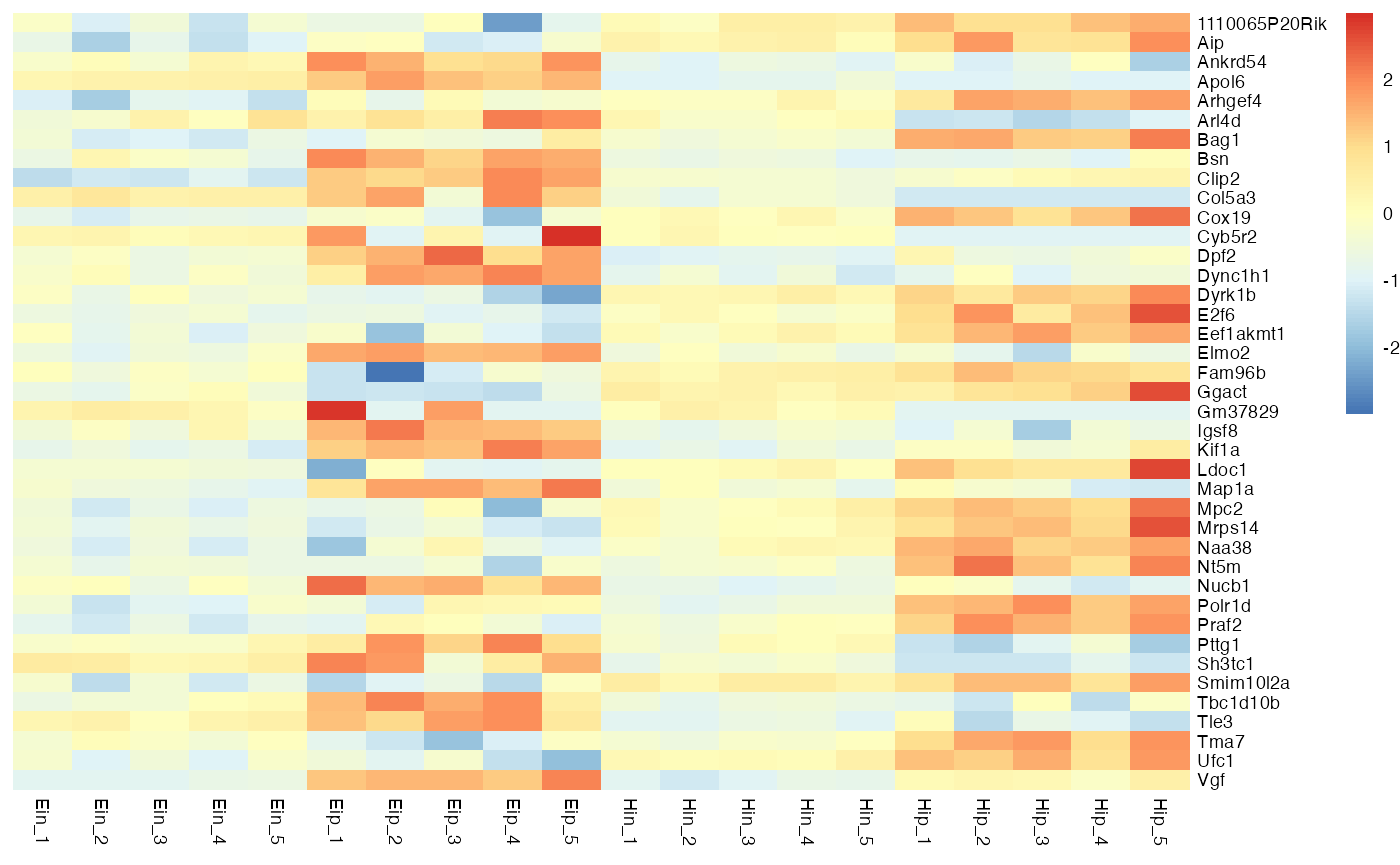
Ordering
Rows and columns in the heatmap will appear in the same order as in the tidy data frame used as input. For example, to order rows and columns alphabetically, just use the dplyr::arrange().
bro_data_exprs %>%
  arrange(external_gene_name, sample) %>%
  bro_plot_heatmap(rows = external_gene_name,
                   columns = sample,
                   values = expression,
                   scale = "row"
)
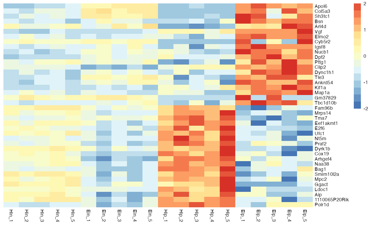
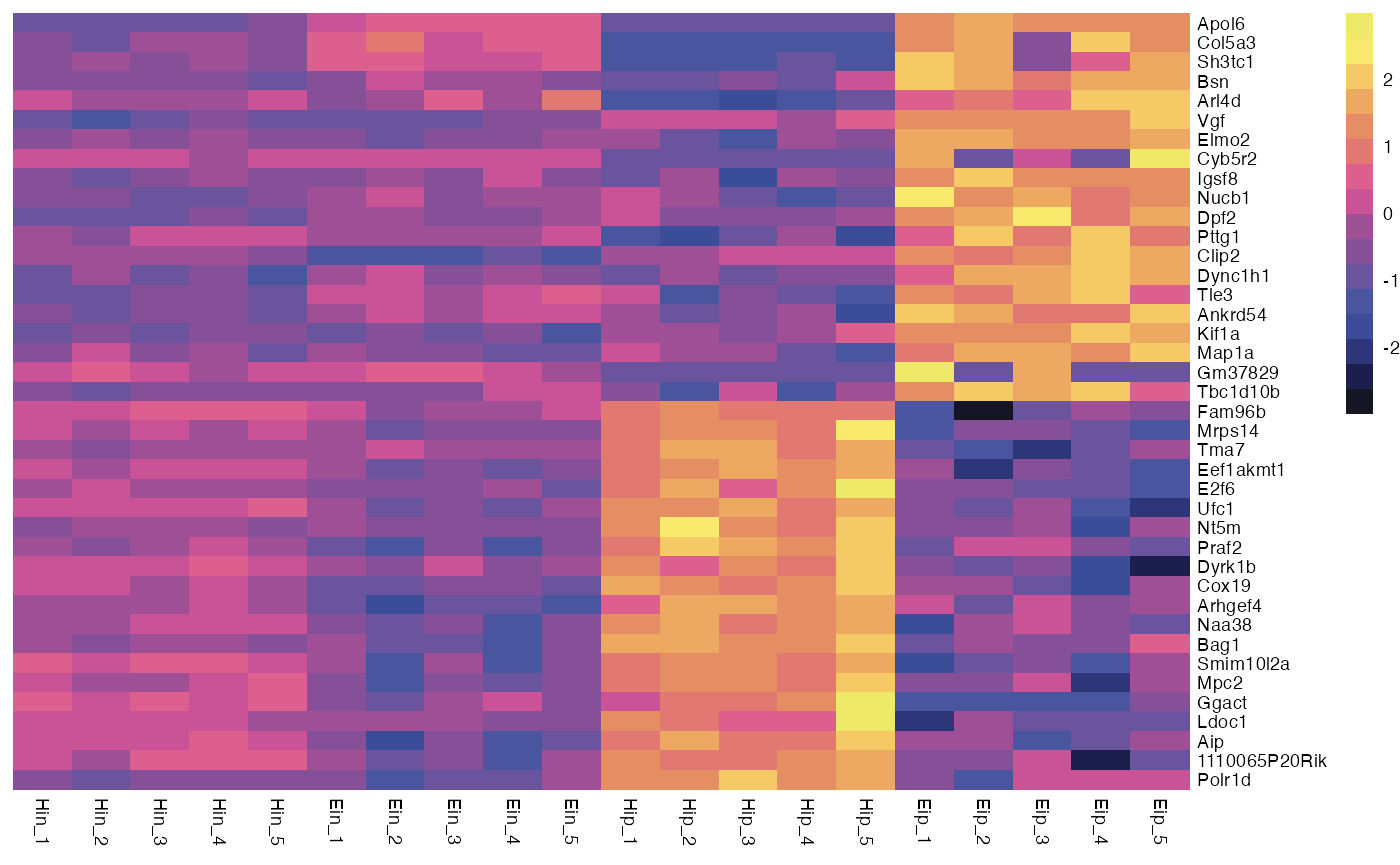
Color legend
You can customize the number of colors color_scale_n and also the minimum and maximum values of the color legend, color_scale_min and color_scale_max.
bro_plot_heatmap(bro_data_exprs,
                 rows = external_gene_name,
                 columns = sample,
                 values = expression,
                 scale = "row",
                 color_scale_n = 16,
                 color_scale_min = -2,
                 color_scale_max = 2
)
Of course, you can also replace the color legend altogether.
bro_plot_heatmap(bro_data_exprs,
                 rows = external_gene_name,
                 columns = sample,
                 values = expression,
                 scale = "row",
                 color = c("#161523","#1C1E4C","#2D3679","#3B4D98","#49569F","#69549D",
                           "#855097","#9E4F96","#CA5296","#DC5F8E","#E17872","#E58D63",
                           "#EDA962","#F5CA66","#F9E96C","#EEE969")
)
Annotations
Annotations can be added for both rows and columns via ann_row and ann_col, respectively. Just specify the corresponding variables in the tidy data frame. If you want more then one variable for annotation just combine them by c(var1, var2, var3).
bro_plot_heatmap(bro_data_exprs,
                 rows = external_gene_name,
                 columns = sample,
                 values = expression,
                 ann_col = c(sample_type, condition, group),
                 ann_row = c(is_immune_gene, direction),
                 scale = "row",
                 color_scale_n = 16,
                 color_scale_min = -2,
                 color_scale_max = 2
)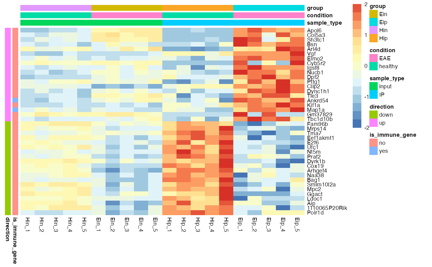
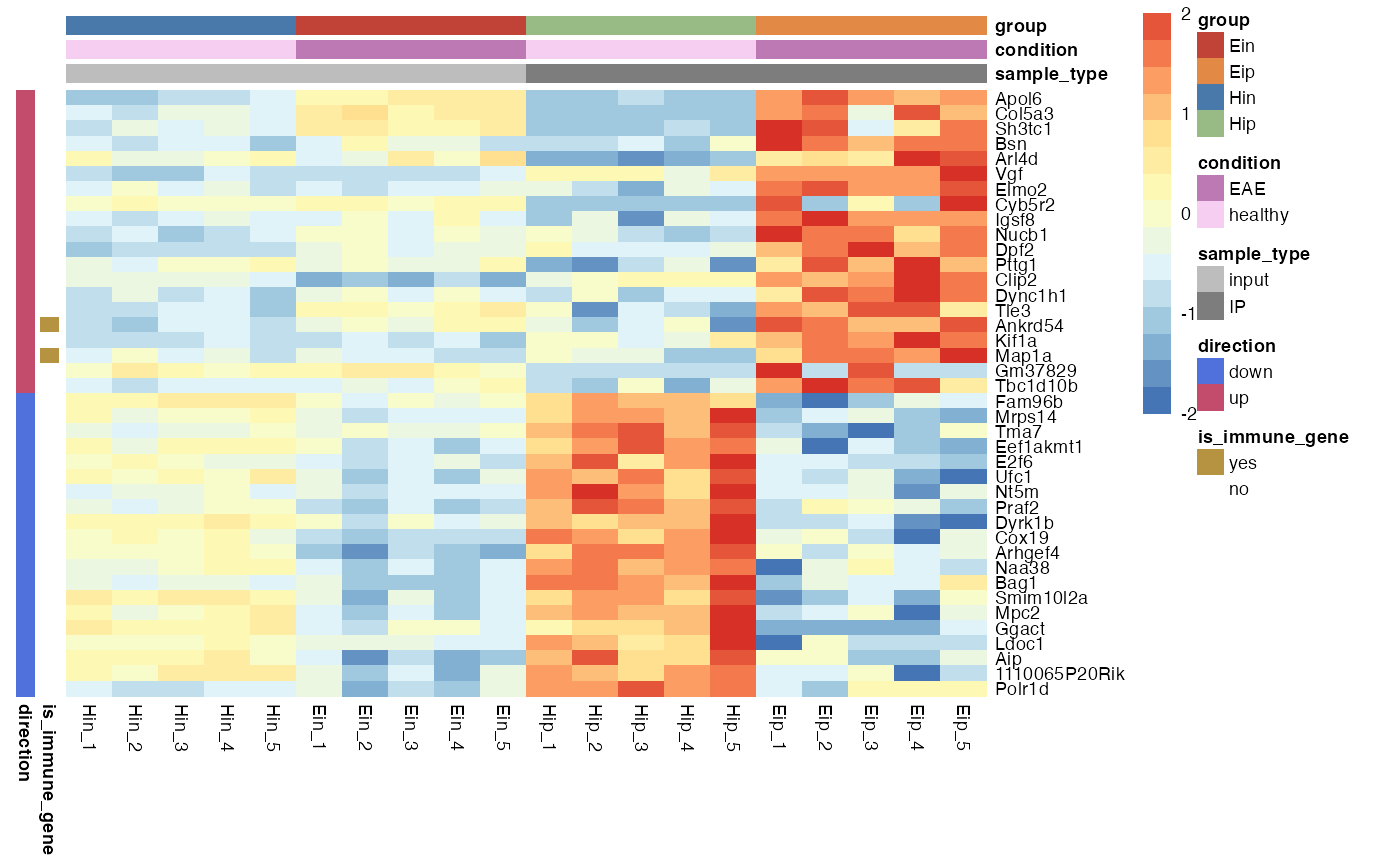
Customize annotations colors
You can provide a list of named vectors to take control over the annotations colors ann_colors.
ann_colors <- list(
  condition = c(EAE = "#BD79B4", healthy = "#F5CEF2"),
  group = c(Ein = "#C14236", Eip = "#E28946", Hin = "#4978AB", Hip = "#98BB85"),
  sample_type = c(input = "#BDBDBD", IP = "#7D7D7D"),
  direction = c(down = "#5071DC", up = "#C34B6B"),
  is_immune_gene = c(yes = "#B69340", no = "#FFFFFF")
)

bro_plot_heatmap(bro_data_exprs,
                 rows = external_gene_name,
                 columns = sample,
                 values = expression,
                 ann_col = c(sample_type, condition, group),
                 ann_row = c(is_immune_gene, direction),
                 scale = "row",
                 color_scale_n = 16,
                 color_scale_min = -2,
                 color_scale_max = 2,
                 ann_colors = ann_colors
)
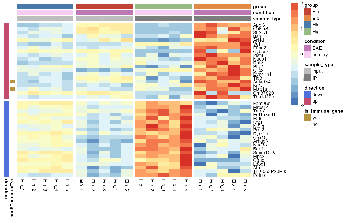
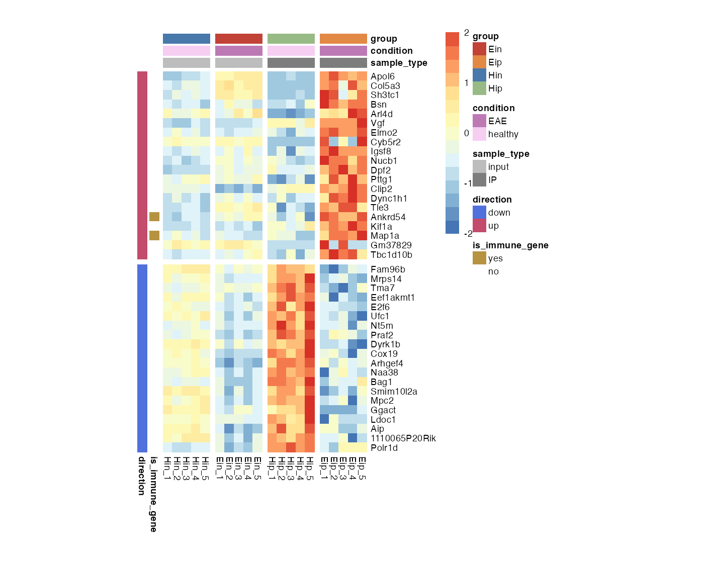
Gaps
Gaps can be added by specifying data frame variables that should be used to generate the gaps. Only one variable can be chosen for gaps_row and one for gaps_col.
bro_plot_heatmap(bro_data_exprs,
                 rows = external_gene_name,
                 columns = sample,
                 values = expression,
                 ann_col = c(sample_type, condition, group),
                 ann_row = c(is_immune_gene, direction),
                 scale = "row",
                 color_scale_n = 16,
                 color_scale_min = -2,
                 color_scale_max = 2,
                 ann_colors = ann_colors,
                 gaps_row = direction,
                 gaps_col = group
)
Fix cell dimensions
You can fix the cell dimensions via the cellwidth and cellheight parameters.
bro_plot_heatmap(bro_data_exprs,
                 rows = external_gene_name,
                 columns = sample,
                 values = expression,
                 ann_col = c(sample_type, condition, group),
                 ann_row = c(is_immune_gene, direction),
                 scale = "row",
                 color_scale_n = 16,
                 color_scale_min = -2,
                 color_scale_max = 2,
                 ann_colors = ann_colors,
                 gaps_row = direction,
                 gaps_col = group,
                 cellwidth = 7,
                 cellheight = 7
)
Write to file
You can use the parameter filename to write the heatmap to file.
bro_plot_heatmap(bro_data_exprs,
rows = external_gene_name,
columns = sample,
values = expression,
filename = "my_heatmap.pdf"
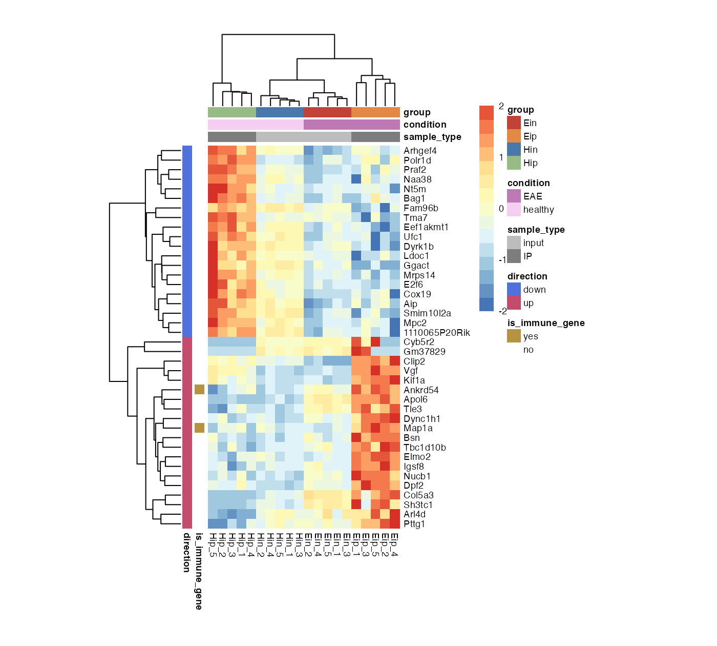
)More features
There are even more features like clustering and dendrograms implemented in pheatmap::pheatmap(). All parameters that are not directly evaluated by bro_plot_heatmap() will be automatically passed to pheatmap::pheatmap().
bro_plot_heatmap(bro_data_exprs,
                 rows = external_gene_name,
                 columns = sample,
                 values = expression,
                 ann_col = c(sample_type, condition, group),
                 ann_row = c(is_immune_gene, direction),
                 scale = "row",
                 color_scale_n = 16,
                 color_scale_min = -2,
                 color_scale_max = 2,
                 ann_colors = ann_colors,
                 cellwidth = 7,
                 cellheight = 7,
                 cluster_rows = TRUE,
                 cluster_cols = TRUE
)
What’s under the hood?
bro_plot_heatmap() takes the tidy data frame and the additional arguments and does the data wrangling needed to satisfy pheatmap::pheatmap(). By setting return_data = TRUE you can get a glimpse at the result of the data wrangling.
bro_plot_heatmap(bro_data_exprs,
                 rows = external_gene_name,
                 columns = sample,
                 values = expression,
                 ann_col = c(sample_type, condition, group),
                 ann_row = c(is_immune_gene, direction),
                 gaps_row = direction,
                 gaps_col = group,
                 return_data = TRUE
)
#> $m
#>                   Hin_1     Hin_2     Hin_3     Hin_4     Hin_5     Ein_1
#> Apol6          2.203755  2.203755  2.660558  2.649534  3.442740  5.030997
#> Col5a3         3.623289  2.950514  3.883794  3.821838  3.486696  5.347029
#> Sh3tc1         3.094325  3.945669  3.721781  4.071979  3.569361  5.758298
#> Bsn            9.594692  9.481155  9.663027  9.621492  9.254889  9.549501
#> Arl4d          6.379306  5.795141  5.767258  5.991696  6.256381  5.513601
#> Vgf            7.386505  6.861794  7.266003  7.738055  7.575901  7.385140
#> Elmo2          8.964594  9.191505  8.996498  9.091161  8.877599  8.940428
#> Cyb5r2         3.846136  4.181117  3.778346  3.687823  3.817430  4.242324
#> Igsf8          8.357730  8.182801  8.386692  8.557224  8.453666  8.401367
#> Nucb1          8.472584  8.486825  8.245469  8.378464  8.521781  8.934631
#> Dpf2           8.209568  8.291422  8.374594  8.442385  8.289120  8.723934
#> Pttg1          8.137118  7.937426  8.404651  8.352276  8.469586  8.156889
#> Clip2          8.754678  8.733512  8.694684  8.715489  8.554136  7.846969
#> Dync1h1       11.602393 11.942333 11.551018 11.851763 11.346086 12.000915
#> Tle3           7.289507  7.292232  7.546951  7.607970  7.198383  8.416004
#> Ankrd54        5.867274  5.619651  6.048261  5.986635  5.665235  6.463674
#> Kif1a         12.437160 12.581432 12.410019 12.770907 12.579293 12.524093
#> Map1a         13.417764 13.772932 13.446422 13.530706 13.201875 13.563318
#> Gm37829        3.911792  4.704230  4.474480  3.796259  4.124560  4.462020
#> Tbc1d10b       8.827458  8.456042  8.726761  8.808308  8.656032  8.639146
#> Fam96b         7.835157  7.517774  7.957167  8.045903  8.081315  7.301972
#> Mrps14         9.088216  8.681238  8.922262  8.876584  9.258166  8.500837
#> Tma7           6.811239  6.566974  6.949656  6.908019  7.116900  6.844333
#> Eef1akmt1      7.099069  6.641980  7.059650  7.361731  7.093585  6.844333
#> E2f6           8.896741  9.150440  8.964573  8.654886  8.829067  8.465089
#> Ufc1           9.416171  9.296585  9.387115  9.321553  9.659070  8.983176
#> Nt5m           7.804291  7.995676  8.048851  8.187596  7.817257  7.979595
#> Praf2          8.381444  8.195282  8.537184  8.777298  8.709678  7.945404
#> Dyrk1b         6.547531  6.467346  6.543533  6.825701  6.429647  6.044776
#> Cox19          7.678025  7.837444  7.647610  7.914175  7.539717  7.035425
#> Arhgef4       10.341459 10.299102 10.306279 10.569326 10.301059  9.643109
#> Naa38          6.916126  6.660135  7.287685  7.481177  7.418356  6.397601
#> Bag1          10.574157 10.398226 10.500136 10.594572 10.454331 10.484227
#> Smim10l2a      7.894974  7.404043  7.899221  7.873827  7.571691  6.825633
#> Mpc2           9.548895  9.108171  9.299191  9.511867  9.882313  8.854007
#> Ggact          6.739533  6.404070  6.492079  6.258252  6.592570  5.137649
#> Ldoc1          5.691651  5.692469  5.816111  6.162898  5.531716  5.095964
#> Aip           10.641707 10.466733 10.643964 10.766897 10.318114  9.478571
#> 1110065P20Rik  5.302977  5.024172  5.703733  5.750027  5.616628  4.939347
#> Polr1d         8.553674  8.320197  8.445705  8.649320  8.645059  8.669130
#>                   Ein_2     Ein_3     Ein_4     Ein_5     Hip_1     Hip_2
#> Apol6          5.314412  5.372403  5.536960  5.645714  2.203755  2.203755
#> Col5a3         5.970917  5.200783  5.380863  5.414576  2.203755  2.203755
#> Sh3tc1         5.628464  4.943715  5.004403  5.505737  2.203755  2.203755
#> Bsn           10.336688  9.978072  9.823801  9.465946  9.427566  9.401769
#> Arl4d          5.697178  6.555629  6.031178  7.073764  4.493476  4.561038
#> Vgf            7.394351  7.393358  7.676219  7.781865  9.049624  9.300449
#> Elmo2          8.777253  8.986457  8.935158  9.130373  9.052209  8.822092
#> Cyb5r2         4.330928  3.906655  4.122089  4.180508  2.203755  2.203755
#> Igsf8          8.692153  8.365600  8.955830  8.445110  8.056258  8.517292
#> Nucb1          9.042499  8.533012  8.976209  8.717655  9.020879  8.859275
#> Dpf2           8.901595  8.525343  8.685763  8.714508  9.131351  8.539024
#> Pttg1          8.262570  8.153131  8.188274  8.504625  7.394518  7.203414
#> Clip2          8.004669  7.980647  8.256524  7.994040  8.739036  8.891307
#> Dync1h1       12.203191 11.700997 12.095691 11.835714 11.587370 12.117493
#> Tle3           8.538112  8.166341  8.529046  8.603207  8.275674  6.664542
#> Ankrd54        6.806487  6.350472  7.038793  6.907131  6.425222  5.510484
#> Kif1a         12.726740 12.468208 12.601176 12.239755 13.040172 13.008885
#> Map1a         13.414518 13.374582 13.211265 13.125640 13.819813 13.550660
#> Gm37829        4.909113  4.627398  4.316214  3.711095  2.203755  2.203755
#> Tbc1d10b       8.861327  8.849873  9.273811  9.404788  8.528672  8.086715
#> Fam96b         6.356636  7.066705  6.689155  7.317450  8.756578  9.641596
#> Mrps14         7.942847  8.427253  8.188274  8.342835  9.832043 10.285114
#> Tma7           7.254255  7.016478  6.784851  7.150363  8.193745  8.906015
#> Eef1akmt1      5.794391  6.338816  5.536960  6.228244  8.030265  8.767910
#> E2f6           8.290413  8.496872  8.685763  8.219487  9.891710 10.713109
#> Ufc1           8.333873  8.823020  8.300294  9.017444 10.487858 10.344933
#> Nt5m           7.665054  7.938917  7.891876  7.775837  9.325486 10.060336
#> Praf2          7.549944  8.088675  7.608173  8.004387  9.811593 10.681098
#> Dyrk1b         5.269735  6.254461  5.536960  5.797272  7.627413  7.060328
#> Cox19          6.759376  7.038219  7.089617  7.033880  8.961613  8.730623
#> Arhgef4        9.170855  9.791434  9.706727  9.408687 10.840547 11.551055
#> Naa38          5.556250  6.373502  5.536960  6.210416  9.131351  9.457031
#> Bag1           9.941392 10.009557  9.893316 10.284755 11.955751 12.001475
#> Smim10l2a      5.357711  6.662247  5.608986  6.363402  8.146133  8.967404
#> Mpc2           8.011377  8.600253  8.140910  8.714508 10.555920 10.918746
#> Ggact          4.966731  5.839785  6.082447  5.382831  6.480152  7.029922
#> Ldoc1          5.075229  5.147621  4.891888  4.792294  7.698471  7.090106
#> Aip            8.360385  9.399647  8.734433  9.125643 11.376675 12.298776
#> 1110065P20Rik  3.904594  4.587228  3.606475  4.742274  6.839297  6.254633
#> Polr1d         8.024701  8.301193  8.211385  8.803094  9.974441 10.069697
#>                   Hip_3     Hip_4     Hip_5     Eip_1     Eip_2     Eip_3
#> Apol6          2.619196  2.203755  2.203755  7.207838  8.418188  7.505587
#> Col5a3         2.203755  2.203755  2.203755  6.900971  7.825300  3.719267
#> Sh3tc1         2.203755  2.932447  2.203755  8.434457  8.051111  3.719267
#> Bsn            9.520877  9.264847 10.194225 11.871814 11.444950 11.083346
#> Arl4d          4.205448  4.438281  4.835291  6.552481  7.099169  6.695912
#> Vgf            9.204563  8.585649  9.514597 10.931662 11.184191 11.176536
#> Elmo2          8.525198  9.101038  8.908268  9.970747 10.031208  9.857982
#> Cyb5r2         2.203755  2.203755  2.203755  6.728107  2.203755  4.266641
#> Igsf8          7.506240  8.486750  8.279999  9.808985 10.289182  9.777884
#> Nucb1          8.391101  8.083832  8.309137 10.775210 10.149783 10.243176
#> Dpf2           8.502422  8.623033  8.841703  9.802469 10.066092 10.665406
#> Pttg1          7.689547  8.076149  7.097184  8.709842  9.649422  9.101513
#> Clip2          9.086007  9.180797  9.213187  9.966868  9.802079  9.933866
#> Dync1h1       11.481329 11.809939 11.841209 12.494681 13.397535 13.314656
#> Tle3           7.493971  7.238095  6.794339  9.548462  9.224495  9.958299
#> Ankrd54        5.953090  6.674710  4.889054  8.830037  8.418188  7.749207
#> Kif1a         12.765709 12.826279 13.523318 13.965006 14.222354 14.103765
#> Map1a         13.495391 12.977465 12.929212 14.300342 14.931126 14.920673
#> Gm37829        2.203755  2.203755  2.203755  9.246378  2.203755  7.156942
#> Tbc1d10b       9.274336  7.894408  9.084301 10.594685 11.215603 10.784057
#> Fam96b         9.161602  9.031911  8.667046  5.036369  2.203755  5.396467
#> Mrps14        10.446139 10.017238 11.681903  7.627301  8.184126  8.491745
#> Tma7           9.061288  8.231774  9.120360  6.303794  5.908813  5.188813
#> Eef1akmt1      9.211133  8.529567  9.025541  6.593407  4.392886  6.345960
#> E2f6           9.538148 10.242673 11.423428  8.411804  8.471214  8.139536
#> Ufc1          10.697065 10.061670 10.952405  8.825760  8.418188  8.995318
#> Nt5m           9.326266  8.935445  9.889655  7.749807  7.741421  8.020793
#> Praf2         10.220552  9.916178 10.587568  7.854334  8.953492  8.737433
#> Dyrk1b         7.726716  7.583559  8.789252  5.259213  5.096047  5.396467
#> Cox19          8.382811  8.730516  9.530145  7.438400  7.557424  6.911790
#> Arhgef4       11.459819 11.299810 11.583997 10.404160  9.822626 10.452586
#> Naa38          8.684764  8.869578  9.539394  4.530752  6.623996  7.505587
#> Bag1          11.721443 11.641706 12.408304  9.989989 10.520580 10.411887
#> Smim10l2a      8.992131  8.145087  9.397410  5.152236  5.908813  6.345960
#> Mpc2          10.697065 10.431086 11.836423  8.511054  8.665741  9.427408
#> Ggact          7.197444  7.499866  9.511467  4.342894  4.392886  4.266641
#> Ldoc1          6.651752  6.691598  9.855504  2.203755  5.560057  4.266641
#> Aip           11.120444 11.242921 12.433740 10.157616 10.213406  8.914373
#> 1110065P20Rik  6.208129  6.760435  7.016961  4.342894  4.392886  5.188813
#> Polr1d        10.414774  9.896324 10.241586  8.667443  8.119152  9.158861
#>                   Eip_4     Eip_5
#> Apol6          7.116522  7.692020
#> Col5a3         8.444539  6.795068
#> Sh3tc1         5.605475  7.439714
#> Bsn           11.585093 11.489941
#> Arl4d          8.637639  8.449852
#> Vgf           10.864963 12.160344
#> Elmo2          9.872046 10.027214
#> Cyb5r2         2.203755  8.632506
#> Igsf8          9.726716  9.615808
#> Nucb1          9.657107 10.140765
#> Dpf2           9.674827 10.185692
#> Pttg1          9.793121  9.031047
#> Clip2         10.594067 10.339874
#> Dync1h1       13.595866 13.354095
#> Tle3          10.125012  8.835462
#> Ankrd54        7.836834  8.773737
#> Kif1a         14.682213 14.385192
#> Map1a         14.732255 15.269623
#> Gm37829        2.203755  2.203755
#> Tbc1d10b      11.092944  9.728544
#> Fam96b         6.765439  6.373782
#> Mrps14         7.705013  7.481524
#> Tma7           6.103697  7.052702
#> Eef1akmt1      5.605475  5.145525
#> E2f6           8.268975  7.898976
#> Ufc1           8.014395  7.418346
#> Nt5m           7.008741  8.073099
#> Praf2          8.359427  7.718482
#> Dyrk1b         4.170949  3.253924
#> Cox19          6.103697  7.385686
#> Arhgef4       10.072506 10.171403
#> Naa38          6.299870  5.807935
#> Bag1          10.317786 11.193410
#> Smim10l2a      5.270378  6.996101
#> Mpc2           7.116522  9.034560
#> Ggact          4.170949  5.197424
#> Ldoc1          4.170949  4.389168
#> Aip            9.044393  9.930596
#> 1110065P20Rik  2.203755  4.190115
#> Polr1d         9.149524  9.089636
#>
#> $ann_row
#>               is_immune_gene direction
#> Apol6                     no        up
#> Col5a3                    no        up
#> Sh3tc1                    no        up
#> Bsn                       no        up
#> Arl4d                     no        up
#> Vgf                       no        up
#> Elmo2                     no        up
#> Cyb5r2                    no        up
#> Igsf8                     no        up
#> Nucb1                     no        up
#> Dpf2                      no        up
#> Pttg1                     no        up
#> Clip2                     no        up
#> Dync1h1                   no        up
#> Tle3                      no        up
#> Ankrd54                  yes        up
#> Kif1a                     no        up
#> Map1a                    yes        up
#> Gm37829                   no        up
#> Tbc1d10b                  no        up
#> Fam96b                    no      down
#> Mrps14                    no      down
#> Tma7                      no      down
#> Eef1akmt1                 no      down
#> E2f6                      no      down
#> Ufc1                      no      down
#> Nt5m                      no      down
#> Praf2                     no      down
#> Dyrk1b                    no      down
#> Cox19                     no      down
#> Arhgef4                   no      down
#> Naa38                     no      down
#> Bag1                      no      down
#> Smim10l2a                 no      down
#> Mpc2                      no      down
#> Ggact                     no      down
#> Ldoc1                     no      down
#> Aip                       no      down
#> 1110065P20Rik             no      down
#> Polr1d                    no      down
#>
#> $ann_col
#>       sample_type condition group
#> Hin_1       input   healthy   Hin
#> Hin_2       input   healthy   Hin
#> Hin_3       input   healthy   Hin
#> Hin_4       input   healthy   Hin
#> Hin_5       input   healthy   Hin
#> Ein_1       input       EAE   Ein
#> Ein_2       input       EAE   Ein
#> Ein_3       input       EAE   Ein
#> Ein_4       input       EAE   Ein
#> Ein_5       input       EAE   Ein
#> Hip_1          IP   healthy   Hip
#> Hip_2          IP   healthy   Hip
#> Hip_3          IP   healthy   Hip
#> Hip_4          IP   healthy   Hip
#> Hip_5          IP   healthy   Hip
#> Eip_1          IP       EAE   Eip
#> Eip_2          IP       EAE   Eip
#> Eip_3          IP       EAE   Eip
#> Eip_4          IP       EAE   Eip
#> Eip_5          IP       EAE   Eip
#>
#> $gaps_row
#> [1] 20
#>
#> $gaps_col
#> [1]  5 10 15